Semiautomated Handwriting Fonts
One of the things which really drives me is resourcing underserved languages, particularly in terms of digital inclusion. Some of the most exciting times of my missionary years was when I was working for the Asia Pacific Sign Language Development Association, delivering digital content for Deaf communities, and the most exciting part of my work now is knowing that what I do has the potential to bring additional expressiveness to digitally underserved languages. But as well as digital side, what about the analogue side? Is there a potential for fonts to be useful in language development, increasing literacy and promoting the use of minority or emerging scripts within their communities?
Surely there is. We learn to read and write our native scripts through carefully constructed material - primers and letter formation charts:
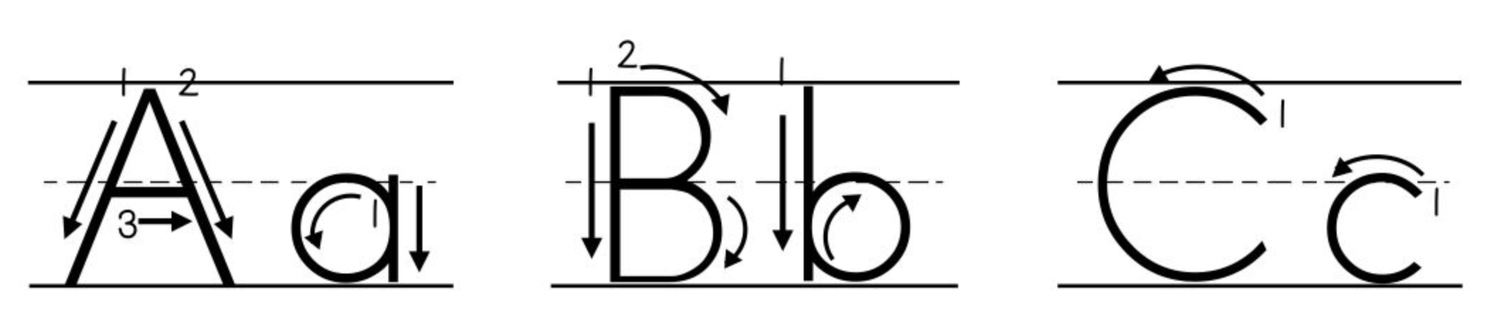
And these are, or certainly can be, expressed as fonts. Fred Brennan’s technically amazing FRB American Cursive font is a wonderful example, with dotted forms, direction arrows, stroke order numbers and so on. But that’s a lot of work.
All of which goes to explain why I was sitting down late on Saturday night with a drink and a packet of crisps thinking “I wonder if we could automate - or at least semi-automate - the production of letter formation fonts given an existing font for a script.” You know, the way that people do.
And it turns out we can. So let’s get started.
First we want to look at renderings of our letters in ways that we can manipulate using numpy/scipy tools, and the way to do that is with a library I wrote a while back called tensorfont. Let’s load up a font and make it big:
from tensorfont import Font

f = Font("NotoSerifKannada-ExtraBold.ttf", 250)
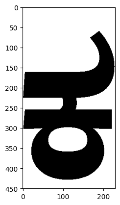
And now let’s take a letter and have a look at it as a binary matrix:
import numpy as np
import matplotlib.pyplot as plt
c = f.glyph("ka_kannada").as_matrix(binarize=True)
plt.ylim((450, 0))
plt.imshow(c, cmap="binary")
<matplotlib.image.AxesImage at 0x29adc1630>
The next thing we need to do is work out the letter’s skeleton, variously called its “heartline” or “midline”. How do we do that? Well, I guess we kind of erode the letter from its edges pixel by pixel until we hit another pixel being eroded in another direction, but… urgh, this is hard. Surely someone’s already done this.
scikit indeed has a library called scikit-image, and one of its packages is all about doing clever things with the morphology of an image. This gives us not just one but three methods for skeletonizing an image. Let’s compare them:
from skimage.morphology import medial_axis, skeletonize
fig, (ax1, ax2, ax3) = plt.subplots(1,3)

# Medial axis transform
skel, distance = medial_axis(c, return_distance=True)
dist_on_skel = distance * skel
ax1.imshow(dist_on_skel/30 + c, cmap="binary")
ax1.set_title("Medial axis transform")
ax1.set_ylim((450, 0))

# Zhang
skeleton = skeletonize(c)
ax2.imshow(skeleton + c, cmap="binary")
ax2.set_title("Zhang's algorithm")
ax2.set_ylim((450, 0))

# Lee
skeleton_lee = skeletonize(c, method='lee')
ax3.imshow(skeleton_lee/256 + c, cmap="binary")
ax3.set_title("Lee's algorithm")
ax3.set_ylim((450, 0))
(450.0, 0.0)
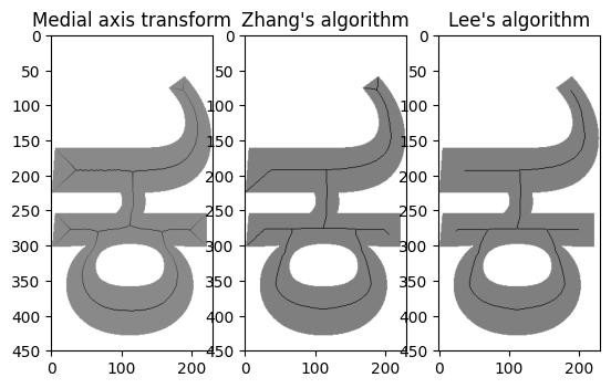
Well, this is all right, isn’t it? The medial distance transform and the default skeletonization algorithm (“A fast parallel algorithm for thinning digital patterns”, T. Y. Zhang and C. Y. Suen, Comm. ACM 27:3) both do a decent job but seem to descend into corners more than we would like for our purposes. (Would be very interesting for creating templates for stone cutting, perhaps…) But the “Lee” algorithm (“Building skeleton models via 3-D medial surface/axis thinning algorithms”, T.-C. Lee, R.L. Kashyap and C.-N. Chu, Computer Vision, Graphics, and Image Processing, 56(6):462-478, 1994) gives us pretty much what we want for most glyph shapes.
You see, to me this is the lovely thing about programming in the 21st century. Despite what big companies and their job interviewers would have you believe, most of the time you don’t need be an absolute data structures and algorithms wizard to be a programmer. Real computer scientists have not only worked out a lot of the clever ways to do things, but they’ve also provided sample code which has made its way into accessible libraries in your favourite programming language. (Or if not, a programming language you can read and translate into your favourite programming language.) It’s not the 1960s any more, and for 99% of the stuff you need to do as a programmer you don’t have to derive it all from first principles any more. Being a programmer today is 10% inspiration and 90% plumbing together code that other people have already written.
Anyway, on with the show. We’ve got our skeleton and we want to get a bunch of open curves out of it. Problem here: we have an image of a set of lines, and we need to split up those lines and turn each one of them into a Bezier curve. How do we know which part of the image belongs to which line? I guess we start at one and trace its neighbours until we get to a junction with another line, and…
I’m kidding! We just search for “skeleton analysis python” and the power of Google directs us to the skan library which does it all for us.
from skan import Skeleton, draw, summarize
sk = Skeleton(skeleton_lee)
labels = sk.path_label_image()
data_masked = np.ma.masked_where(labels == 0, labels)
plt.imshow(data_masked, interpolation = 'none', vmin = 0)
plt.ylim((400, 50))
(400.0, 50.0)
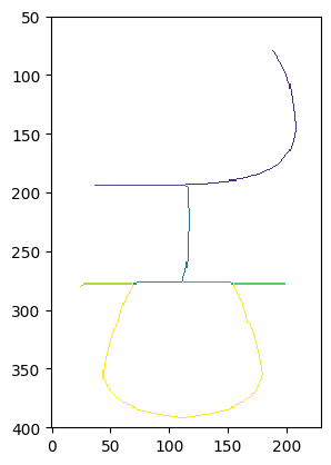
That’s almost good enough. The skeleton is a bit rough, and we’ve split the middle stroke into three separate lines, which isn’t what we want. As a later refinement, we could check the position and direction of each stroke and merge together any strokes which meet at a point and continue in the same direction and tangent. But to do that we need to get our Beziers, so let’s do that. We’ll use the path-fitting algorithm in my Beziers.py library. (Did I write a clever path-fitting algorithm? Of course not, I stole it from Inkscape.) We deliberately use a high error value to smooth the curve a bit, and use the tidy method to add extrema.
from beziers.path import BezierPath
from beziers.point import Point
fig, ax = plt.subplots()
paths = []
for i in range(len(sk.paths_list())):
    bp1 = BezierPath.fromPoints([Point(x,y) for y,x in sk.path_coordinates(i)], error=200)
    bp1.tidy(maxCollectionSize=0, lengthLimit=50)
    bp1.plot(ax)
    paths.append(bp1)
ax.set_ylim(450,0)
ax.set_aspect("equal")
plt.show()
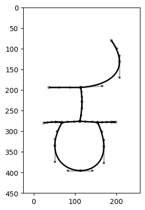
Well, it’s OK. I’m hoping to replace my Inkscape-based path fitting code with Raph Levien’s improved Bezier fitting algorithm, not least because this will improve the continuity of the returned curves, but again the way to do this is to wait for the clever people to write the code and then translate it into our favourite language.
OK, we’re nearly there. Now we have some open curves, but if we’re going to use them in a font, we want to turn them into closed curves. Once again, there’s a library for that! Matthew Blanchard’s MFEK/math has some Rust code for constant width stroking, dotting and dashing and varioud other kinds of path creation from a UFO glyph object. So let’s turn our paths into a UFO glyph, and expand them:
from beziers.path.representations.fontparts import FontParts

g = Glyph()
for p in paths:
    FontParts.drawToFontpartsGlyph(g, p)

from ufostroker import constant_width_stroke

constant_width_stroke(g, 20)
Before pulling them out again to take a look at:
paths = BezierPath.fromDrawable(g)
fig, ax = plt.subplots()

for p in paths:
    p.plot(ax, fill=True, drawNodes=False, color="black")
ax.set_ylim(450,0)
ax.set_aspect("equal")
plt.show()
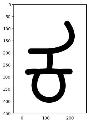
And there we go. Let’s put all the steps together:
from ufoLib2.objects import Glyph, Font
f, (ax1, ax2, ax3, ax4) = plt.subplots(1, 4, sharey=True, figsize=(15, 15))

ax1.imshow(c, cmap="gray")
ax1.set_aspect("equal")

ax2.imshow(skeleton_lee/255 + c, cmap="gray")
ax2.set_aspect("equal")

ax3.imshow(c, cmap="gray")
paths = []
for i in range(len(sk.paths_list())):
    bp1 = BezierPath.fromPoints([Point(x,y) for y,x in sk.path_coordinates(i)], error=200)
    bp1.tidy(maxCollectionSize=0, lengthLimit=50)
    bp1.plot(ax3)
    paths.append(bp1)
ax3.set_ylim(450,0)
ax3.set_aspect("equal")

g = Glyph()
for p in paths:
    FontParts.drawToFontpartsGlyph(g, p)
from ufostroker import constant_width_stroke

constant_width_stroke(g, 30)
paths = BezierPath.fromDrawable(g)
for p in paths:
    p.plot(ax4, fill=True, drawNodes=False, color="black")

ax1.set_ylim(500,0)
ax1.set_xlim(-50,250)
ax1.set_xlabel("Render")
ax2.set_ylim(500,0)
ax2.set_xlim(-50,250)
ax2.set_xlabel("Skeletonize")
ax3.set_ylim(500,0)
ax3.set_xlim(-50,250)
ax3.set_xlabel("Fit Beziers")
ax4.set_ylim(500,0)
ax4.set_xlim(-50,250)
ax4.set_aspect("equal")
ax4.set_xlabel("Expand stroke")
plt.show()
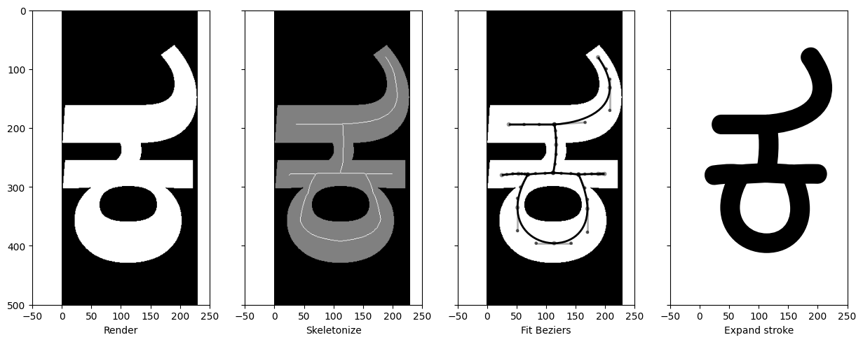
It’s not bad. It’s not perfect, but I’m not expecting it to be perfect; there’ll still need to be manual intervention to ensure the strokes have the correct number and are in the correct order so that stroke order annotations can be added later. There will still need to be some touching up on the Beziers and joining the appropriate curves together. And that’s OK - any time you do font stuff, you probably want human intervention to be the final pass. But it’s sure a lot easier to be able to start with something than to have to draw all those curves from scratch.